Image segmentation with deep learning
Note: This tutorial follows the Jupyter Notebook here. Use it to follow along.
Deep learning has been around for quite some time, but its popularity has surged in recent years due to its ability to learn complex patterns from data. One of its key applications in computer vision and image analysis is image segmentation, where deep learning models are used to partition an image into meaningful regions.
This is particularly useful in 3D-imaging, where the additional spatial dimension makes it challenging for humans to visualize structures effectively. Typically, 3D images are viewed as a series of 2D cross-sections, which allows for traditional visualization but complicates the task of extracting or labelling specific objects or regions. This is where deep learning-based segmentation can be especially beneficial, as it automates and enhances the process.
A widely used deep learning model for image segmentation is U-Net. Since its introduction in 2015, U-Net has undergone numerous adaptations, including versions designed for handling 3D image data. One such implementation is available in the MONAI Python library, which is specifically designed for medical imaging applications. To further simplify the use of these deep learning tools, the qim3d library provides easy to use functionality, enabling users to quickly train 3D U-Net architectures on their datasets.
A brief introduction to U-Net
Before diving into the code, it’s useful to establish a basic understanding of how the U-Net architecture works and why it is effective for segmentation tasks.
U-Net is a type of convolutional neural network (CNN) specifically designed for image segmentation. The model follows an encoder-decoder structure:
Encoding (Downsampling) – The network first extracts features by applying a series of convolutions and downsampling operations (e.g., strided convolutions) to capture important spatial patterns in the image.
Decoding (Upsampling) – The extracted features are then upsampled to generate a segmentation mask, reconstructing the spatial resolution while maintaining key details.
Skip Connections – U-Net incorporates skip connections between corresponding layers in the encoder and decoder paths, helping to retain fine-grained spatial information and improve segmentation accuracy.
In the 3D U-Net implementation, there are a few key differences compared to the original 2D version:
3D Convolutions – Instead of 2D convolutions, the network applies 3D convolutions, allowing it to process volumetric data directly.
Strided Convolutions for Downsampling – In MONAI's implementation, strided convolutions are used at the beginning of each convolutional block for downsampling, rather than max pooling at the end of the block as in the original U-Net.
Customization – The MONAI implementation is highly configurable, allowing users to tailor it to specific use cases. We encourage readers to explore these options further.
This introduction provides the foundation for understanding U-Net and its 3D variant. Next, we will explore how to implement and train a 3D U-Net model for segmentation using MONAI and qim3d.
Opening the Jupyter Session
Before we start coding, we should consider where we want the code to run. Deep learning can use a lot of memory, since large amounts of operations must be performed in order to improve the model weights. Additionally, the training may take a long time, running on a personal computer. Therefore, we can use the DTU HPC, and run the code in a Jupyter Notebook. First start by navigating to the Jupyter Launcher.
Here we can determine the amount of resources we need for the project. Remember to be conservative, when you request computing resources. A good baseline could be:
- 4 CPUs
- 16 GB Memory
- 8 hour Wall time
- Use of a GPU (e.g.
gpua100)
These resources can be fetched by following this link.
Once the Jupyter session is launched, navigate to a workspace, and create a new Jupyter Notebook.
Preparing the data
First we need to make the necessary imports and set up a base path for the deep learning project. The functions that prepare the data for model training expects files to follow this structure:
dataset
├── train
│   ├── images
│   │   ├── 1
│   │   ├── 2
│   │   └── (...)
│   └── labels
│       ├── 1
│       ├── 2
│       └── (...)
└── test
    ├── images
    │   ├── 3
    │   └── (...)
    └── labels
        ├── 3
        └── (...)
The first step is therefore to create these directories, such that the data can be placed there. Run the following code to define a base path:
# Import packages
import qim3d
import os

# Base path for the dataset directory
base_path = os.path.join(os.path.expanduser("~"), "qim3d-unet-dataset")
print(f"Dataset directory: {base_path}")

# Option to remove already existing files in the dataset directory
clean_files = True
Now we can run the following code to generate the folder structure in the base path:
# Create directories
print("Creating directories:")

for folder_split in ["train", "test"]:
    for folder_type in ["images", "labels"]:
        # Define the folder path and create it
        path = os.path.join(base_path, folder_split, folder_type)
        os.makedirs(path, exist_ok=True)
        print(path)

# if the option for clean_files is true, remove the paths inside the folders (if they exist)
if clean_files:
    for root, dirs, files in os.walk(base_path):
        for file in files:
            file_path = os.path.join(root, file)
            os.remove(file_path)
We should now have a folder named qim3d-unet-dataset which contains two folders, train and test in which each contains a folder for images and labels. If you already have images and labels for your project, please skip the next step, and instead populate the folders with your data. The data is loaded with qim3d.io.load() and is therefore expected in a 3D image format. Additionally, we recommend you name the images and corresponding labels similarly, as the files are matched up using alphabetical sorting.
Since we dont have data easily available, we will generate some using the qim3d.generate module.
# Specify the number of training and testing samples
num_train = 5
num_test = 1

# Specify the number of objects in each collection volume
num_volumes = 10

# Generate training and testing samples
print(f"Generating {num_train} training and {num_test} testing samples with {num_volumes} objects each:")

for idx in range(num_train + num_test):

    # Determine the folder split (train or test)
    if idx < num_train:
        folder_split = "train"

    else:
        folder_split = "test"

    # Generate volumes of shape 128x128x128
    vol, label = qim3d.generate.volume_collection(
        num_volumes=num_volumes,
        collection_shape=(128, 128, 128),
        min_shape = (30, 30, 30),
        max_shape = (40, 40, 40),
        min_volume_noise=0.04,
        max_volume_noise=0.08,
        seed=idx
    )

    # Convert N + 1 labels (each object and background) into 2 labels (any object and background)
    label = (label > 0).astype(int)

    # Save volume
    qim3d.io.save(os.path.join(base_path, folder_split, "images", f"{idx + 1}.tif"), vol, compression = False, replace = True)

    # Save label
    qim3d.io.save(os.path.join(base_path, folder_split, "labels", f"{idx + 1}.tif"), label, compression = False, replace = True)
This will generate 6 volumes, where we use 5 for training (and validating) and 1 for testing. The volumes are of size (128x128x128) and are saved into the newly created folders. We recommend you to load a volume using qim3d.io and validate that it exists. This also allows you to visualize it and see what we are working with. Load and visualize the first element of the training set with:
# Load in the first generated volume
vol_path = '/qim3d-unet-dataset/train/images/1.tif'
vol = qim3d.io.load(vol_path)

# Visualize it
qim3d.viz.volumetric(vol)
Creating the model and dataloaders
Now that the data is ready, we can prepare a model for the segmentation.
Model architecture
The qim3d library contains multiple premade models, that make it easy to use. If you need something specific, this can also be created using the UNet class. The premade architectures have the following options:
- Name....... - No. of layers - No. of channels
- xxsmall.... - 2 layers - (4,8)
- xsmall...... - 2 layers - (16,32)
- small........ - 3 layers - (32, 64, 128)
- medium... - 3 layers - (64, 128, 256)
- large......... - 5 layers - (64, 128, 256, 512, 1024)
- xlarge....... - 6 layers - (64, 128, 256, 512, 1024, 2048)
- xxlarge..... - 7 layers - (64, 128, 256, 512, 1024, 2048, 4096)
Since we are using a small and rather simple dataset, we will use the smallest model.
# Define the 3D UNet model
model = qim3d.ml.models.UNet(size = 'xxsmall')
Augmentations
Since we dont have a lot of training data, we can use augmentations to introduce more variance to the training data and thereby make the model more robust. The qim3d library offers a pre-defined augmentation of three different levels.
- light
- Performs a 90 degree rotation on the images with 100% probability?
- moderate
- Performs a 90 degree rotation on the images with 100% probability?
- Performs a flip along one of the two first axes each with 30% probabilty.
- Performs random Gaussian smoothing with probability of 10%.
- Performs affine transformation with translation up to 10% of the volume size and be scaled with up to 10% of the image size with 50% probability.
- heavy
- Performs a 90 degree rotation on the images with 100% probability?
- Performs a flip along one of the two first axes each with 70% probabilty.
- Performs random Gaussian smoothing with probability of 30%.
- Performs affine transformation with translation up to 20% of the volume size, be scaled with up to 40% of the image size and sheared shear angle between ±15° with 50% probability.
For the generated dataset we will only need light augmentation. We define the augmentation with the following code:
# Define augmentation
augmentation =  qim3d.ml.Augmentation(
    resize = 'crop',
    transform_train = 'light',
    transform_validation = None,
    transform_test = None,
    )
Dataloaders
We previously made a train and a test split for the data. While we set the model up to train on the data, we make an additional split such that we have a validation set. This set is used to validate the model performance and optimize the parameters. We can use qim3d.ml.prepare_dataset() to generate the train-, validation- and test set.
# Define dataset splits
train_set, val_set, test_set = qim3d.ml.prepare_datasets(
    path = base_path,
    val_fraction = 0.2,
    model = model,
    augmentation = augmentation
    )
This will split the training set such that 20% is used for validation. Additionally this sets up augmentation to be used on the training data. Lastly we need to create data loaders to ensure compatability with PyTorch and set up the iteration throught the data.
# Define data loaders
train_loader, val_loader, test_loader = qim3d.ml.prepare_dataloaders(
    train_set = train_set,
    val_set = val_set,
    test_set = test_set,
    batch_size = 1,
    num_workers = 4,
    )
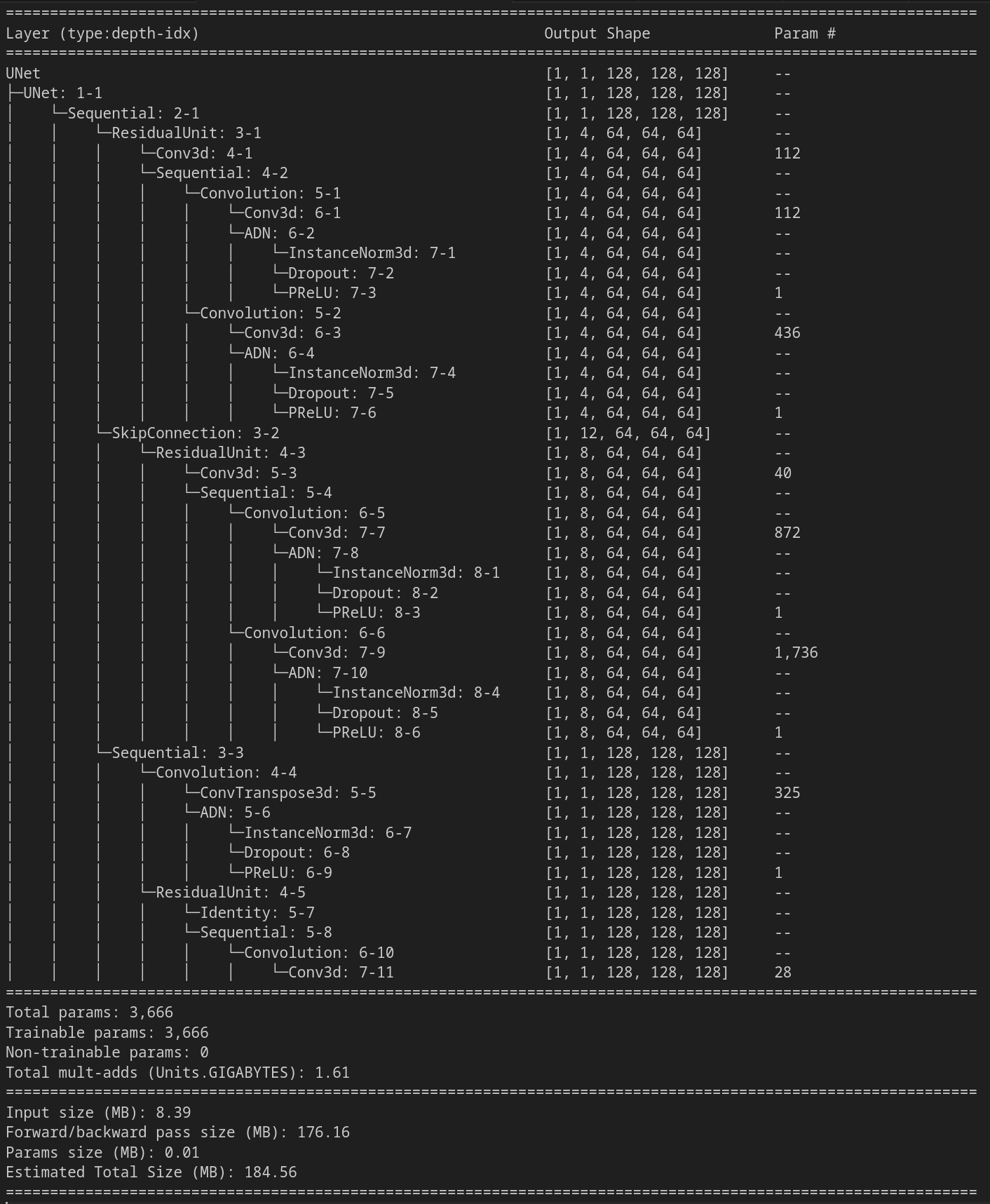
Since we don't have a lot of data, we use batch size of 1. When we started the Jupyter session we requested 4 CPUs, so lets use them all with 4 workers. Lastly, we can summarize the model and dataloader with qim3d.ml.model_summary():
# Get model summary
summary = qim3d.ml.model_summary(model, train_loader)
print(summary)
This will print a summary:
Training the model
We are now almost ready to train the model. First we need to define the hyper parameters, that define how the model learns. These parameters include
- Number of epochs
- Learning rate
- Loss function
- Weight decay
There are a number of different things to consider when choosing hyperparameters, so for now, try with the following:
# Define hyperparameters
hyperparameters = qim3d.ml.Hyperparameters(
    model = model,
    n_epochs = 30,
    learning_rate = 1e-2,
    loss_function = 'DiceCE',
    weight_decay = 1e-3,
    )
Finally, we have everything ready for training. Using qim3d.ml.train_model() we can start training with the specified hyperparameters. This function also allows us to save the trained model and plot the progression of the loss. The loss quantifies the error using the loss function wich is why we should see the loss go down through multiple epochs.
# Train model
qim3d.ml.train_model(
    model = model,
    hyperparameters = hyperparameters,
    train_loader = train_loader,
    val_loader = val_loader,
    checkpoint_directory = base_path,
    plot = True,
    )
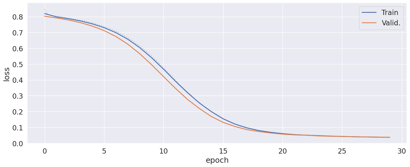
Once the training has finished, we should see our validation loss starting at 0.8 and ending at 0.03. We see that our model has converged nicely, with the training loss similar to the validation loss. A typical sign of overfitting, would be if the training- and validation loss were very different. This could maybe be mitigated with changes to the hyper parameters or augmentations.
Testing the model
Now that we have trained the model, we need to check how it performs on unseen data. This is what we use the test set for.
First we apply the model on the test set and extract the results. After this we can visualize the ground truth, prediction and difference between the two:
# Apply the trained model to test set
results = qim3d.ml.test_model(
    model = model,
    test_set = test_set,
    )

# Get results for the first test image
volume, target, pred = results[0]

# Define the slices we wish to visualize
slice_positions = [10, 31, 63, 95, 110]

# Visualize the target segmentation (ground truth label) and the predicted segmentation
print(f"Ground truth label of test image:")
qim3d.viz.slices_grid(target, num_slices=5, slice_positions=slice_positions, display_figure=True)

print(f"Predicted segmentation of test image:")
qim3d.viz.slices_grid(pred, num_slices=5, slice_positions=slice_positions, display_figure=True)

print(f"Difference (prediction - ground truth)")
qim3d.viz.slices_grid(pred-target, num_slices=5, slice_positions=slice_positions, value_min=-1, value_max=1, color_map="coolwarm")
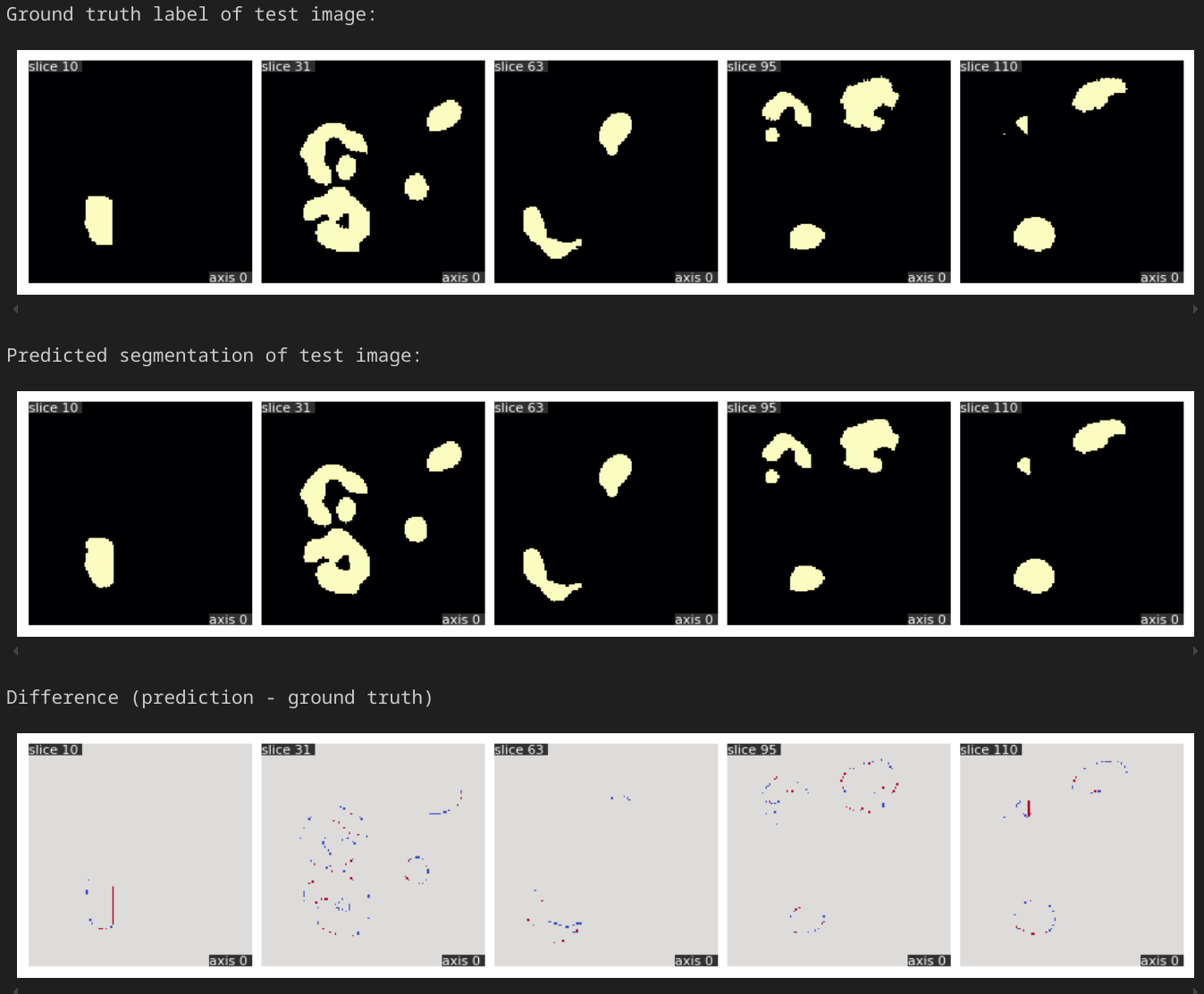
Here we see that the ground truth and model prediction have little differences through different layers. This looks pretty good, though for real use, we should train the model on more data.
This concludes this tutorial. We have covered data formatting and generation, model- and agumentation- and hyperparameter definition along with training and testing. By following these steps, you should be able to use qim3d to apply similar techniques to your own data.